Calibration Transfer in Spectroscopy: Why Models Break When Instruments Change

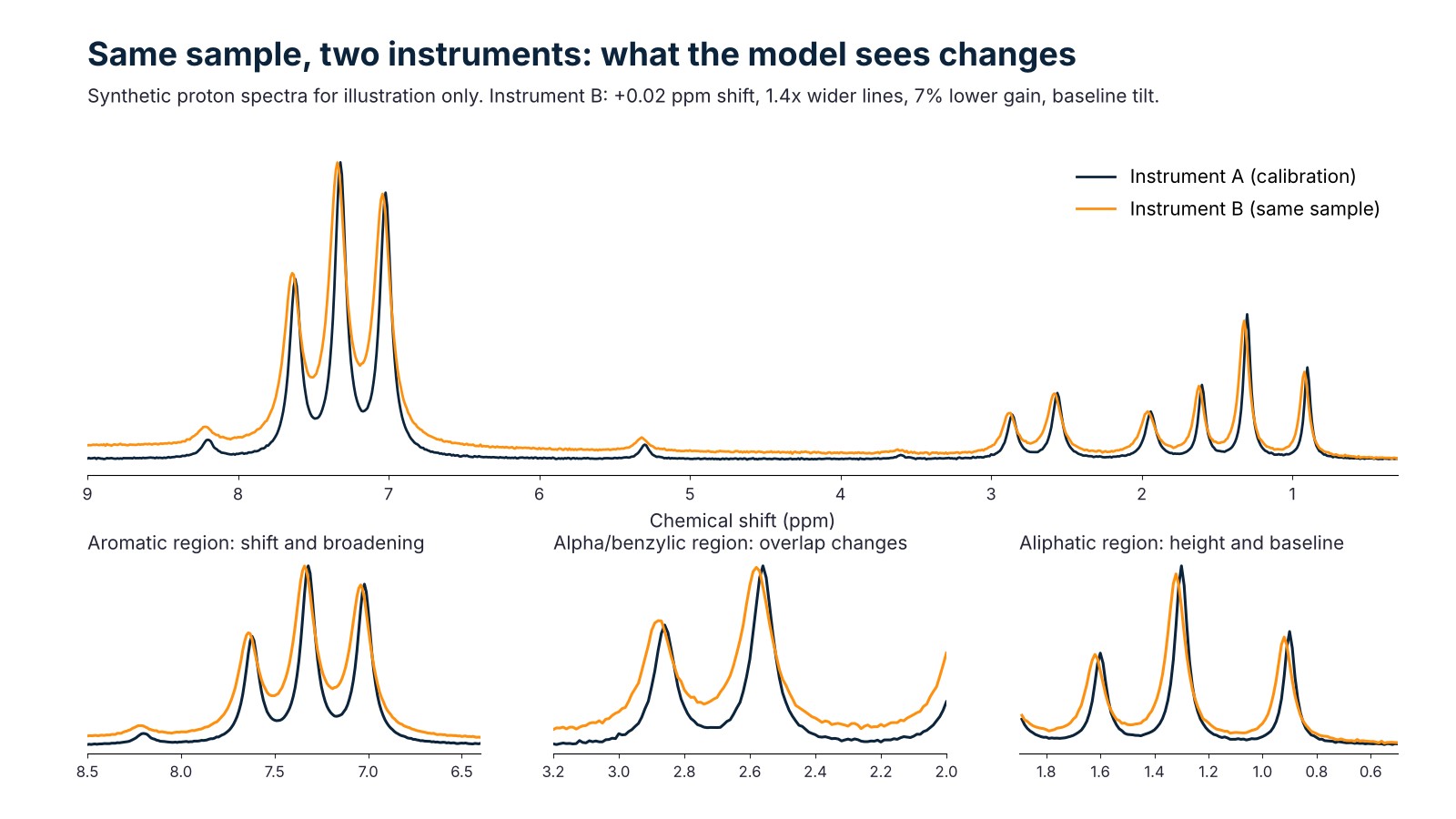
A calibration model learns the link between spectra and a property on one instrument. A second instrument records the same sample with a different line shape, shift, gain and baseline, so the model receives an input it has not seen and its predictions drift. Calibration transfer corrects that gap, or avoids it, before the model is used for decisions.

Last reviewed: 26 October 2026.

TL;DR

• The chemistry does not change, the input does. Peak position, resolution, line shape, gain and baseline differ between instruments, and a model trained on one set of spectra reads another set differently.
• Four families of fixes exist. Slope and bias correction of predictions, spectral standardization (direct and piecewise direct), recalibration on the second instrument, and invariance built in at training time. Each needs different data from the lab.
• In a simulated example, an uncorrected transfer gave 4.8 times the error of the original instrument. Corrections that used 20 paired samples brought it to 1.2 to 1.4 times. The data are synthetic and show the mechanism, not a benchmark.
• A transfer is a validation task. Independent paired samples, acceptance limits agreed in advance and the reference method as the judge decide whether a model has moved safely.
• Foundation models change where the effort goes. Training across many instruments and field strengths is designed to reduce transfer work, but whether it does so for your two instruments is a test, not an assumption.

Why does a model that works on one instrument fail on the next?

A partial least squares (PLS) model maps a spectrum, treated as a list of numbers, to a property. It has no concept of an instrument. It knows only what the calibration spectra looked like, so anything that changes how the same chemistry appears in the spectrum moves the input outside what the model has seen.

Workman and Mark’s review of calibration transfer lists the usual sources: differences in instrument response between a parent and a child instrument, long-term drift, temperature, scattering differences and unmodeled variation in the samples themselves. Feudale and co-authors give the broader review of the methods that address them.

In proton NMR, four effects matter most:

• Field strength and resolution. Signal dispersion grows with field: about 60 Hz per ppm at 60 MHz against 400 Hz per ppm at 400 MHz. Because J couplings are fixed in hertz, a multiplet spans more ppm at lower field and neighbouring signals overlap more easily, as Nanalysis explains. A 43 MHz and a 60 MHz benchtop record different overlap patterns for the same molecule.
• Line shape. Shim quality and sample properties such as viscosity change linewidth. A model trained on narrow lines meets wider ones.
• Referencing and shift. Small offsets between instruments, or between days, move peaks by a few hundredths of a ppm. On a grid with 0.01 ppm spacing that is a few points, enough to change which variables carry the signal.
• Gain, phase and baseline. Receiver settings, processing and baseline correction change the intensity scale and the background.

None of these changes the chemistry. All of them change what the model reads.

What are the main ways to transfer a calibration?

Transfer methods differ mainly in what they ask of the laboratory: spectra of shared samples, reference-method results, or neither.

Approach	What the lab provides	What it corrects	Main limit
Slope and bias correction	Predictions of the same samples on both instruments	A constant offset and scale in the predicted values	Cannot repair shifts or line-shape changes that affect different variables differently
Direct standardization (DS)	Spectra of transfer samples measured on both instruments	One global linear map from the second instrument’s spectra to the first	Assumes a single linear relation holds across the whole spectrum
Piecewise direct standardization (PDS)	Spectra of transfer samples measured on both instruments	Local linear maps: each variable of the first instrument is predicted from a window of variables on the second	More settings to choose (window width, latent variables); the transfer samples must span the range
Recalibration on the second instrument	New samples with reference-method results, measured on the second instrument	Whatever the new samples cover	Needs reference results; the cost grows with every property and instrument
Invariance at training time	Data from several instruments in the calibration set or in pre-training	Differences represented in the training data	Cannot cover differences it has never seen

PDS, introduced by Wang, Veltkamp and Kowalski in 1991, is still the commonly used method that newer approaches are compared against in the Workman and Mark review. Brown’s chapter on transfer of multivariate calibration models reviews the wider set of methods.

NMR transfer across field strengths has been tested. In a 2022 study in Analytical Chemistry, Lindner and co-authors moved a PLS calibration for lignin molecular weight from a 600 MHz instrument to benchtop instruments at 43 and 60 MHz using PDS, canonical correlation analysis and an extreme learning machine auto-encoder. The study listing reports validation errors as low as about 1.2 times those of the original calibration. That is one property, one sample type and one team’s setup. It shows that transfer can work despite a large resolution gap, not that it will for your samples.

What does a transfer look like in a worked example?

The example below is a simulation, so every assumption is on the page. It shows how the methods behave, not how any product performs.

Assumptions

• Eight synthetic components (aromatic, polyaromatic, olefinic, benzylic, naphthenic, CH2, CH3 and heteroatom-bound hydrogens) with Lorentzian lines on a 0 to 10 ppm grid of 1,000 points.
• An illustrative property in arbitrary units, built from the component amounts plus a reference-method error of 0.4 (standard deviation). The standard deviation of the property across samples is about 3.5.
• Instrument A: line half-width 0.035 ppm, small per-spectrum variation in shift and width. Instrument B: half-width 0.050 ppm (about 1.4 times wider), an average shift of +0.02 ppm with more spectrum-to-spectrum scatter, 7% lower gain, a baseline tilt and somewhat higher noise.
• PLS model with 5 latent variables built on 100 samples measured on A. Evaluation on 60 further samples measured on both instruments.
• Transfer samples chosen from the calibration set with the Kennard-Stone algorithm and measured on both instruments. PDS uses a window of 17 points (plus or minus 0.08 ppm) and 2 latent variables per window.
• 20 simulated experiments with different random draws. Results are mean and standard deviation of the root mean square error of prediction (RMSEP).

Results

Scenario	RMSEP (mean ± SD)	Relative to A on A
Model built on A, tested on A	0.50 ± 0.06	1.0
Model built on A, tested on B, no correction	2.39 ± 0.26	4.8
Slope and bias correction, 20 transfer samples	0.69 ± 0.09	1.4
PDS, 20 transfer samples	0.62 ± 0.07	1.2
New model on B, 100 reference-labelled samples	0.59 ± 0.07	1.2
New model on B, 40 reference-labelled samples	0.66 ± 0.10	1.3
New model on B, 20 reference-labelled samples	0.79 ± 0.10	1.6
New model on B, 10 reference-labelled samples	1.04 ± 0.23	2.1

Three points follow from the table.

1. The uncorrected model fails by a large margin. Its error is about six times the reference-method error, although the chemistry is identical on both instruments.
2. Paired samples recover most of the gap. With 10 transfer samples the corrected errors were 0.72 (slope and bias) and 0.68 (PDS); with 40 they were 0.68 and 0.61. PDS was a little better than slope and bias correction here, and neither needed new reference-method results.
3. Rebuilding costs reference data. The rebuilt model reached the same error as the transferred ones only with roughly 40 labelled samples. In a crude or transformer oil lab, each label is a reference-method test, such as a titration, a distillation or a Karl Fischer run.

What the simulation does not show. It has no matrix effects, no new sample types, and its instrument differences are stable and smooth, which is what these methods handle best. Real gaps are less tidy, so the sample counts above are not a guide for a real transfer. They show the shape of the trade-off: paired spectra are cheaper than new reference results, and they correct only what the transfer samples span.

How many transfer samples, and which ones?

There is no universal number. The useful rules are qualitative.

• Span the range. Transfer samples should cover the property range and the spectral variation you expect in routine work, including the extremes. A selection algorithm such as Kennard-Stone picks samples that are spread out in the spectral space, which is what the simulation used.
• Measure back to back. A sample that changes between runs, for example by losing volatiles or taking up water, adds a difference that is not instrument-related. Measure on both instruments close together, or use stable standards.
• Keep some samples out. The samples used to fit the transfer cannot be used to judge it. Hold back independent paired samples for validation.
• Expect the gap to move. A new probe, a shim change or a magnet service can reopen a transfer that was closed.

How should a lab validate a transferred model?

Treat the transferred model as a new method on the second instrument.

1. Quantify the gap first. Measure a handful of samples on both instruments and compare the spectra and the predictions. If the predictions differ by a constant, slope and bias may be enough. If peaks have moved or broadened, they will not be.
2. Choose the method by what you can afford. If you can run the same samples on both instruments but cannot spend reference tests, use a standardization method. If reference tests are available, recalibration is an option.
3. Validate on independent paired samples. Run the reference method on samples that were not used to fit the transfer, covering the grades and blends you actually process.
4. Agree acceptance limits in advance, per property, referenced to the reproducibility of the reference method.
5. Flag samples outside the model’s domain and route them to the reference method.
6. Keep checking. Re-test a share of samples with the reference method so drift on either instrument is caught.

For infrared analyzers in petroleum laboratories, ASTM D6122 frames this kind of validation: instrument performance, whether the model applies to each spectrum, and agreement with the primary test method. The practice is written for infrared systems and does not describe a transfer procedure. The same logic is a sensible way to structure the work for any spectroscopic analyzer.

Where Rombo AI fits

Rombo AI builds property models on NMR spectra and benchmarks each property against the customer’s reference method, with acceptance metrics agreed before a pilot starts. Our foundation model is pre-trained on 3.2 million experimental, simulated and benchtop proton spectra, with an objective that pulls together spectra of the same molecule recorded at different field strengths. It is designed to need fewer reference samples per property and to carry across instruments. The evaluation described in that post covers molecular identity tasks such as classification and structure retrieval. It does not report property calibration on crude oil or transformer oil, so it does not by itself show that a given property transfers.

That is why the test belongs on your instruments: paired samples on each, predictions compared with your reference method, acceptance limits agreed first. For a crude oil lab or a transformer oil lab with more than one NMR system or site, a feasibility review starts from your own samples and reference methods, and paired measurements on each instrument belong in the test design. Our posts on multi-instrument compatibility and multi-site deployment describe the architecture; the comparison of lab testing, NIR and high-field NMR covers the alternatives. To test transfer on your own samples, start with a feasibility review.

FAQ

Can a bias correction alone be enough?

Sometimes. If the two instruments give predictions that differ by a constant offset and scale, a slope and bias correction fixes it with a few paired samples. If peaks have shifted or broadened, the error is not constant across the spectrum and the correction leaves part of it in place, as the simulation shows.

Do I have to rebuild the model every time an instrument is serviced?

Not necessarily, but you should check. Run a few paired or reference samples after the service and compare with the validated performance. A small, constant change can be handled by correction; a large or irregular one may justify a new transfer or recalibration.

Does transfer work between high-field and benchtop NMR?

It has worked for at least one property. Lindner and co-authors transferred a lignin molecular weight calibration from 600 MHz to 43 and 60 MHz instruments with errors close to the original, per the study listing. Whether it works for another property depends on whether the information is still resolved at the lower field.

Is NMR easier to transfer than near-infrared?

Part of the problem is easier. A chemical-shift axis referenced to a standard removes much of the wavelength alignment issue that NIR labs know. Line shape, resolution, gain and baseline differences remain, and so does the need to validate against the reference method. Our comparison of lab testing, NIR and high-field NMR covers where each technique fits.

How many reference samples does a new instrument need?

It depends on the property, the sample diversity and the method. In the simulation above, a rebuilt model needed about 40 labelled samples to match transferred ones, while paired samples without reference results got close with 10 to 20. Real data are less forgiving, so plan the count with your own samples and validate on a separate set.

When is recalibration the better choice?

When the instruments differ in ways a transfer cannot span, for example a new sample type or a large change in resolution, or when reference results are cheap and the property set is small. Transfer is most attractive when you have many properties, several instruments or sites, and reference tests are the expensive part.