Spectral Deconvolution: Methods, Pitfalls, and AI

TL;DR

• Spectral deconvolution estimates the components hidden inside a measured signal. It does not create new experimental resolution; it separates contributions only to the extent supported by the data and assumptions.
• Overlap has several causes. Limited linewidth, digital resolution, complex multiplets, co-elution, background, and multiple species can all place distinct signals in the same observed region.
• The method must match the data structure. Peak-shape fitting suits a local 1D envelope, multivariate curve resolution uses variation across samples or time, and GC-MS algorithms can group ions with shared chromatographic profiles.
• A visually smooth reconstruction is not enough. A wrong component count or line-shape model can fit the data while producing biased areas, positions, or identities.
• Validation requires residuals, parameter stability, replicates, standards, and orthogonal evidence. Uncertainty should follow the deconvoluted result into any downstream quantification or identification.
• Learned models can reduce manual initialization and find shoulder peaks, but training coverage and ambiguous overlap still set hard limits.

What spectral deconvolution means

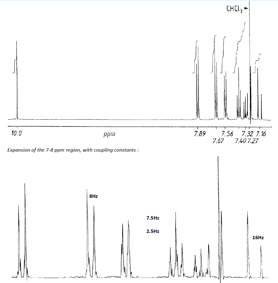
A measured spectrum is often a superposition. At each coordinate x—chemical shift, wavenumber, wavelength, m/z, or retention time—the observed signal can be represented conceptually as:

observed signal = component 1 + component 2 + … + baseline + noise

Spectral deconvolution estimates the number, shape, position, and contribution of those components. Depending on the technique, the output may be a list of fitted NMR lines, pure spectral profiles for co-eluting compounds, zero-charge masses reconstructed from charge-state envelopes, or resolved concentration and spectrum matrices.

Deconvolution does not create independent information. Zero filling may make a Fourier-transformed NMR trace smoother, and background subtraction may remove a nuisance contribution, but neither operation proves that hidden components exist. An incorrect phase or baseline can instead be fitted as an extra component.

A reliable result therefore answers three questions together: What components are proposed? Which assumptions make them distinguishable? What evidence shows that the separation is not a fitting artifact?

Why spectral peaks overlap

Overlap is not one phenomenon, so it has no universal remedy.

Finite linewidth. Every signal has width. In solution NMR, transverse relaxation contributes to the natural linewidth; field inhomogeneity, shimming, acquisition, and processing broaden it further. Mestrelab’s Global Spectral Deconvolution documentation notes both the relaxation limit and instrumental contributions when explaining why many transitions are unresolved inside observed ¹H NMR peaks.

Crowded chemistry. Similar chemical environments may resonate within a narrow range. A multiplet can contain more transitions than the visible local maxima suggest, while strong coupling can produce patterns that are not well represented by a collection of simple first-order lines.

Insufficient sampling or resolution. Short acquisition, wide spectral windows, low resolving power, and coarse digital grids can merge features. Smoothing may suppress noise but also erase shoulders that support a second component.

Multiple analytes. In mixtures, unrelated compounds can contribute signals at the same coordinate. Chromatography helps by adding retention time, yet co-elution can still combine mass spectra. NIST’s AMDIS description shows how a component may be hidden beneath a larger GC peak even when the total-ion chromatogram does not display a distinct maximum.

Background and artifacts. Solvent, water, column bleed, matrix signals, phase errors, ringing, detector saturation, and baseline drift can resemble low-level components. A deconvolution routine will fit artifacts if its model permits them.

Before choosing software, identify the type of overlap. Co-elution, a strongly coupled spin system, and inadequate acquisition each demand different models—and sometimes new data.

Spectral deconvolution methods compared

The main approaches differ in what they assume and which independent dimensions they exploit.

In local curve fitting, the analyst chooses a baseline, component count, peak family, initial positions, widths, and bounds. An optimizer minimizes the difference between measured and reconstructed data; non-negativity and realistic width ranges can constrain the solution.

However, a minimum residual does not guarantee a unique chemical answer. Two close peaks may be practically indistinguishable from one broader peak at the available signal-to-noise ratio. Adding another component will almost always reduce the numerical residual, so model complexity must be justified by reproducible structure in the data rather than improvement alone.

Data-dependent peak models are particularly important for chromatography. A study of high-resolution LC-MS deconvolution found that several peak models produced very similar goodness-of-fit values yet substantially different component areas (Zhang et al., 2014). That is a direct warning for quantification: an excellent fit statistic can coexist with materially different analytical conclusions.

Multivariate methods gain leverage from change. If constituent A varies across samples while B remains constant, their shared region may be separable. Constraints such as non-negativity or unimodality reduce ambiguity, but perfectly covarying components remain difficult to distinguish.

How GC-MS deconvolution groups a hidden component

GC-MS supplies a useful worked mechanism because each scan contains a mass spectrum and each ion has a chromatographic profile.

Imagine two compounds that elute within the same broad total-ion peak. Ions at m/z 111 and 158 rise, maximize, and fall together. An ion at m/z 83 reaches its maximum slightly earlier and has a different profile. Rather than treating the scan at the apparent apex as one pure spectrum, a deconvolution algorithm can assign 111 and 158 to one component and 83 to another.

NIST documents this logic directly for AMDIS: ions that rise and fall together are associated with a component, which is then compared with reference spectra and retention indices. Its detailed spectrum extraction method fits each ion chromatogram to a model component profile with a linear baseline and flags ions that are not explained reliably.

A defensible workflow is:

1. Detect candidate components. Search ion chromatograms for maxima or shoulders rather than relying only on the total-ion trace.
2. Build a model profile. Combine sharp, consistent ions or another representative signal to describe the component’s elution shape.
3. Fit each ion separately. Estimate how much of each ion follows the model profile while accounting for local baseline.
4. Reject or flag incompatible ions. Do not force ions with different maxima or shapes into the extracted spectrum.
5. Reconstruct the component spectrum. Use the fitted contributions at the component maximum.
6. Search and validate. Compare the extracted spectrum with a library, retention information, blanks, replicates, and standards as required.

The output is still conditional. Closely co-eluting compounds can share nearly identical profiles, large background ions can hide a trace component, and the selected model ion can itself be interfered with. Deconvolution improves selectivity when the chromatographic dimension contains enough differential information; it cannot guarantee separation when every observable feature varies together.

Worked example: two overlapping NMR signals

Consider an illustrative ¹H NMR region that appears as one asymmetric envelope with a weak shoulder. The task is to determine whether it contains one distorted resonance or two partially overlapping signals whose areas will be used in a purity calculation.

1. Preserve the original evidence. Inspect the time-domain data, signal-to-noise ratio, digital resolution, phase, baseline, apodization, and any evidence of clipping. Save the raw and processed versions. Deconvolution should not become an irreversible processing step.

2. Fit the simplest adequate model. Start with one physically reasonable line shape and inspect the residual. A broad, sign-changing residual around the shoulder indicates systematic structure that the model has not explained; random residual noise does not.

3. Test a two-component model. Add a second constrained peak with positive area and realistic width. Keep the baseline model fixed unless independent evidence justifies changing it. Compare whether the shoulder position and component areas remain stable across sensible starting values.

4. Challenge the assumptions. Repeat with Lorentzian, Gaussian, and Voigt profiles where appropriate. If the inferred area ratio changes substantially with the peak family while each reconstruction looks good, the result is model-dependent and should not be reported as a precise measurement.

5. Acquire discriminating evidence. Reprocess with a different apodization, repeat the spectrum, change concentration or temperature when chemically appropriate, or use a 2D experiment. A genuine second resonance should behave consistently with the proposed assignment. A spiked standard can test identity and recovery in a targeted workflow.

6. Carry uncertainty forward. If two components are supported but their individual areas remain correlated, report an interval or flag the region as unsuitable for primary quantification. The combined envelope area may be more stable than either fitted component.

This example highlights the central rule: deconvolution is strongest when the model predicts evidence beyond the exact trace used for fitting.

Common pitfalls that create false components

Overfitting the noise. Every added peak improves flexibility. Without a minimum signal criterion, parameter bounds, or complexity penalty, the routine can turn noise excursions into chemically named signals.

Underfitting shoulders. Peak picking based only on local maxima misses smaller peaks dominated by neighbors. The absence of a separate maximum is not proof that only one component exists.

Using the wrong baseline. A curved baseline fitted as a broad peak changes both component count and area. Baseline choices should be evaluated outside the crowded region, not optimized solely to make the residual flat beneath it.

Assuming ideal symmetry. Chromatographic tailing, phase error, exchange, strong coupling, unresolved isotope structure, and detector response can produce asymmetric shapes. Several symmetric components may imitate one asymmetric physical signal.

Ignoring non-identifiability. Different parameter sets can reconstruct the same observed envelope within noise. The Nature Communications paper describing DEEP Picker explicitly excludes synthetic peak pairs that can be represented adequately by one peak, because the data do not support a unique separation.

Validating on reconstruction alone. A fit is an internal consistency check. It is not independent confirmation of component identity, concentration, or chemical assignment.

A validation framework for spectral deconvolution

Validation should be proportional to use. Exploratory peak annotation may tolerate a tentative component. Release testing, impurity quantification, or a high-consequence identification needs predefined criteria and independent evidence. Store the software version, parameters, masks, fitted components, residuals, and manual edits so the decision can be audited.

Where AI changes the deconvolution workflow

Traditional fitting asks an analyst to specify or initialize the component model. Learned methods can infer peak presence and parameters from examples, reducing repetitive manual tuning and improving detection of weak shoulders. DEEP Picker, for instance, uses convolutional layers to classify spectral points and predict position, amplitude, width, and the Gaussian–Lorentzian contribution for overlapping NMR peaks. Its authors also emphasize representative training data, preprocessing quality, and intrinsically ambiguous cases.

Commercial tools are moving in the same direction. Mestrelab’s current Mnova NMR page describes deep-learning peak picking built on its Global Spectral Deconvolution workflow. This is meaningfully different from claiming that a learned model removes the need for validation: the model still encodes a training distribution and can fail on unfamiliar artifacts, line shapes, instruments, or sample types.

Rombo AI’s broader NMR platform takes a foundation-model approach: its public documentation describes a model pre-trained on millions of spectra across materials, conditions, and instruments, rather than a traditional chemometric model rebuilt from scratch for each dataset (Rombo AI foundation model). For deconvolution-heavy workflows, the relevant evaluation is whether learned representations generalize to the laboratory’s actual instruments, samples, overlap regimes, and decision thresholds. A reconstructed spectrum and chemist review remain necessary evidence.

If manual interpretation of crowded NMR data is limiting an industrial workflow, request a Rombo AI feasibility analysis to define the sample, instrument, validation data, and success criteria for a focused pilot.

FAQs

What is spectral deconvolution?

Spectral deconvolution estimates the individual components whose combined signals produce an observed spectrum or chromatographic region. It relies on assumptions about peak shapes, variation, or component behavior and must be validated against raw and independent evidence.

Is deconvolution the same as peak fitting?

Peak fitting is one form of deconvolution. Other approaches use multivariate variation, chromatographic profile correlation, charge-state models, matrix factorization, or learned peak representations rather than fitting one local envelope only.

Can spectral deconvolution separate completely overlapping peaks?

Only when another source of information distinguishes them, such as different behavior across samples, time, ions, or orthogonal experiments. If two components produce indistinguishable observations within noise, no algorithm can recover a unique answer from that dataset alone.

How do I know whether a fitted peak is real?

Look for reproducibility, stable parameters, structured residual improvement, chemically plausible shape, and confirmation in another dimension or experiment. A lower fitting error by itself is insufficient because additional components increase model flexibility.

Does AI make manual spectral review unnecessary?

No. Learned models can automate peak detection and initialization, but performance depends on training coverage and input quality. Analysts still need to inspect ambiguous regions, validate downstream results, and document uncertainty.