How AI Identifies Unknown Compounds from Raw Spectra

TL;DR

• “Raw spectrum” is an imprecise term. An instrument may store a time-domain signal, while an AI model may consume a minimally processed frequency-domain intensity vector, a peak list, or several spectral modalities.
• Preprocessing is part of the identification system. Fourier transformation, phasing, baseline correction, referencing, normalization, and region masking can preserve chemical evidence or silently distort it.
• A learned representation is not an identification. It compresses spectral patterns into features that a downstream model can use for classification, retrieval, substructure prediction, or candidate generation.
• Retrieval and de novo reasoning solve different problems. Retrieval ranks known candidates; structure generation must explore molecules that may be absent from spectral libraries.
• Generalization must be tested across chemistry and acquisition conditions. Instrument, field strength, solvent, concentration, processing, mixtures, and simulated-versus-experimental data can all shift the input distribution.
• The useful output is an auditable hypothesis. Chemists still need raw-data review, alternative candidates, uncertainty, orthogonal measurements, and a decision-appropriate confirmation step.

What counts as a raw spectrum?

AI spectroscopy begins before a neural network sees a number. The first question is which representation actually enters the model.

In Fourier-transform NMR, the instrument first records a time-domain free induction decay (FID). The familiar spectrum appears only after transformation and processing. A vendor directory can also contain acquisition parameters, pulse-sequence information, field strength, temperature, solvent, receiver settings, and processing history. Those metadata affect interpretation even when the model ultimately consumes only an array of intensity values against chemical shift.

Papers often use “raw” to mean that a method accepts a continuous spectrum instead of a manually curated peak list. That does not necessarily mean the network consumes an untouched FID. For example, the NMR2Struct study applies minimal preprocessing to 1D ¹H and ¹³C frequency-domain spectra; its model input is different from a CASE workflow built from manually assigned correlations (Hu et al., ACS Central Science, 2024).

Each representation discards different information. A peak list depends on peak picking; an intensity vector retains unresolved envelopes but depends on alignment and normalization; an FID preserves acquisition-domain information but requires more processing.

A defensible pipeline preserves enough information to move backward through this table. If an analyst cannot connect a candidate to the spectral regions that influenced it, the model has shortened the workflow at the cost of auditability.

The six stages from instrument output to candidate structures

A practical identification system can be divided into six stages. Each has its own failure modes and validation evidence.

1. Ingest data and provenance. The system associates the measurement with technique, acquisition conditions, sample identity, blank, and processing history. File conversion must not separate intensities from interpretive parameters.

2. Check technical quality. Before chemical inference, the pipeline looks for low signal-to-noise, clipping, phase and baseline errors, unstable referencing, solvent dominance, contamination, or mixtures. Artifact tolerance is not proof that data are suitable.

3. Standardize the numerical input. Spectra may be transformed, resampled onto a common axis, scaled, normalized, aligned, or masked. Bruker’s TopSpin materials illustrate how learned methods can operate at this processing layer: official application notes describe deep-learning commands for signal-region detection, phase and baseline correction, and 1D deconvolution (Bruker TopSpin AI algorithms). These functions prepare or expose evidence; they are not by themselves a complete unknown-structure assignment.

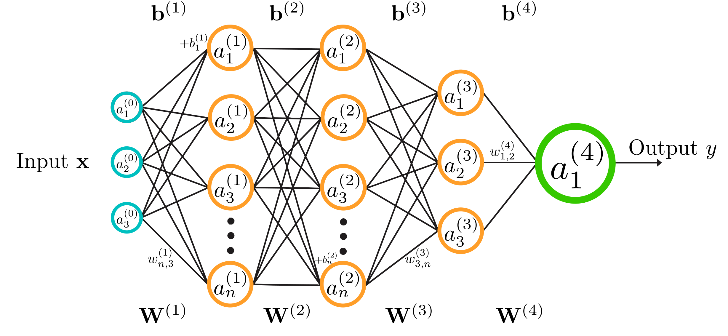
4. Encode spectral patterns. Convolutional networks can detect local peak shapes; transformers can connect distant regions; contrastive learning can place spectra and structures into related numerical spaces. The resulting embedding is a feature vector, not a compound name.

5. Produce chemical hypotheses. A task head can classify a known material, retrieve similar spectra or structures, predict functional groups, rank a supplied candidate set, or generate molecular graphs. The output type determines the strength of the claim. A class prediction such as “aromatic aldehyde” is not equivalent to an exact constitutional structure.

6. Review, challenge, and confirm. The system should expose alternative candidates, supporting regions, violated constraints, confidence behavior, and out-of-domain warnings. The analyst compares predicted and observed evidence and decides whether another NMR experiment, accurate-mass measurement, IR spectrum, separation, authentic standard, or synthesis is needed.

Bruker’s CMC-se page describes the established CASE version of the later stages: NMR constraints are managed, compatible structures are generated, and proposed structures are validated from acquisition through analysis (Bruker CMC-se). The learned pipeline changes how features and candidates are prioritized, but it does not remove the need to test all plausible alternatives.

How models learn spectral features

Hand-coded interpretation starts with explicit rules: a chemical-shift interval suggests an environment, splitting suggests neighboring spins, and a 2D correlation constrains connectivity. These rules are chemically meaningful, but overlap, second-order effects, noise, field strength, and sample conditions make real signals less tidy than reference tables.

A supervised model receives spectra paired with structures, substructures, classes, or peak annotations. Training makes spectral patterns useful for predicting those labels. The model can learn features difficult to specify manually, but also shortcuts tied to a dataset, instrument, simulation engine, or preprocessing convention.

Representation learning separates the shared encoder from the final task. The encoder can reconstruct inputs, align related views, contrast spectrum–structure pairs, or support several tasks. A small head then adapts it to retrieval, classification, denoising, or peak detection. The goal is to avoid relearning the entire spectral front end for every endpoint.

Different outputs require different evidence.

NMR2Struct demonstrates one possible route: a convolutional model predicts simple substructures and a transformer assembles them. In the published test, the correct molecule appeared within the first 15 predictions for 69.6% of simulated-spectrum cases containing up to 19 heavy atoms. The number is informative only with that scope attached; it is not an accuracy promise for arbitrary experimental spectra, larger molecules, mixtures, or different chemical domains (Hu et al., 2024).

More recent work also separates spectral decoding from full identification. MolDeTr uses a detection-transformer design to extract peak, multiplet, chemical-shift, coupling, decay, and proton-count parameters from 1D ¹H NMR spectra. Its reported domain is single-component small molecules with up to ten groups of equivalent spins, trained on simulated spectra augmented with experimental artifacts (Schmid et al., Analytical Chemistry, 2026). Those parameters narrow hypotheses; they do not erase the need for candidate testing.

Worked walkthrough: an unknown reaction side product

Consider an isolated side product from a development reaction. The laboratory has a vendor NMR dataset, a sample record, and a proton spectrum; no trusted reference spectrum is available. The goal is not to let a model guess a name, but to produce the smallest defensible set of hypotheses and the next discriminating action.

Ingestion. The pipeline retains the original FID, field strength, solvent, temperature, pulse program, scan and receiver settings, and processing record. It links the side product to a blank and starting-material spectra.

Quality gate. Checks flag a phase error and dominant residual-solvent region. The system reprocesses the FID under a versioned method, excludes that window from similarity scoring, and preserves both traces. Evidence of a mixture would stop the single-identity workflow.

Representation. The corrected spectrum is mapped to the encoder axis and converted from peak shapes, integrals, separations, and wider relationships into an embedding. Field strength and solvent can be supplied separately from chemical identity.

Hypothesis generation. A retrieval head finds structurally related compounds, while a substructure head proposes several chemical motifs. A formula from high-resolution MS constrains the allowed atoms and degree of unsaturation. The candidate generator returns three constitutional isomers rather than one unexplained answer.

Falsification. The report maps each candidate back to evidence. Candidate A requires a proton environment absent from the spectrum. Candidate B explains most regions but predicts two signals where one unresolved envelope is observed. Candidate C best matches the current data, yet B and C remain too close to distinguish reliably from the 1D spectrum.

Next experiment. The correct output is therefore not “Candidate C confirmed.” It is “C currently ranks first; acquire HSQC and HMBC to distinguish B from C.” The additional correlations test connectivity directly. If the consequence of error is high, the final identity may still require an authentic material or another orthogonal method.

This walkthrough shows where automation creates value: consistent processing, rapid feature extraction, candidate-space reduction, and explicit selection of the next experiment. It also shows the stopping rule. When the data do not distinguish plausible structures, the pipeline must preserve ambiguity.

Generalization limits and validation tests

A model generalizes only across variations represented by its training and validation evidence. “Works on raw spectra” does not answer whether it works on another vendor, field strength, solvent, concentration, pulse sequence, processing chain, molecule class, or mixture regime.

Simulation-to-experiment shift is particularly important. Simulated spectra can provide scale and perfect labels, but their lineshapes, artifacts, noise, and chemical coverage may not reproduce a laboratory. In one SECS analysis of 34 molecules with paired data, a model trained only on simulated spectra achieved 0% top-1 on the experimental ¹H spectra; augmentation raised the reported result to 38.2%, and experimental fine-tuning to 55.8% (Mirza, Patiny, and Jablonka, Nature Communications, 2026). The small, defined subset matters as much as the improvement: it demonstrates the domain gap, not a universal correction recipe.

Validate the complete pipeline, not only the encoder. Freeze file conversion, preprocessing, model, candidate database, thresholds, and reporting version. Use compounds and acquisition conditions excluded from training. Stratify results by instrument, field, solvent, sample type, concentration, and difficulty. Measure candidate recall, top-k ranking, calibration, abstention, and failure detection—not only average top-1 accuracy.

Finally, challenge the system with negatives: mixtures passed as pure compounds, corrupted metadata, shifted references, unseen chemical classes, low signal, and compounds missing from the candidate index. A model that recognizes when not to answer is more useful than one that always returns a confident structure.

The next step: reusable spectral models across instruments

The progression from rules to task-specific models to foundation models is a progression in reuse. A foundation model learns a shared spectral representation before a laboratory supplies every downstream label. Rombo AI describes its broader NMR platform as pre-trained on millions of spectra and designed to generalize across instruments and sample types rather than requiring a separate traditional chemometric recalibration for each instrument.

Spectra AI is a distinct product line for compound identification and full structure elucidation, separate from Rombo AI’s general NMR platform. Rombo reports an analysis workflow of approximately 15 minutes for work that can otherwise take weeks; the claim should be validated against each laboratory’s samples, instruments, file formats, review requirements, and confirmation standard.

For an evaluation, ask to see the path from original files to ranked candidates, the alternatives and evidence behind the result, and performance on held-out spectra from the laboratory’s own operating conditions. Explore Spectra AI for compound identification.

FAQs

Does AI read an NMR spectrum the same way as a chemist?

Not exactly. A chemist uses explicit concepts such as chemical environments, integrals, coupling, symmetry, and connectivity. A model learns numerical features that help a training objective; those features may correlate with chemical concepts but can also capture dataset-specific shortcuts. Evidence mapping helps connect the prediction back to chemistry.

Can AI identify a compound from only a proton NMR spectrum?

It can rank or generate useful hypotheses for some clean, in-domain small molecules, but 1D ¹H data often leave degenerate solutions. ¹³C, 2D NMR, accurate-mass MS, IR, separation, or an authentic standard may be required to distinguish alternatives and support the intended claim.

Is an embedding the same as a fingerprint?

Both are compact representations used for comparison, but a learned embedding is optimized from data and its meaning depends on the training objective. A conventional molecular fingerprint is generated from a known structure using explicit rules. A spectrum embedding starts from the measurement and does not by itself establish that structure.

Why can a model fail on another instrument?

Field strength, resolution, lineshape, noise, referencing, processing, and metadata can change the input distribution. Cross-instrument performance must be demonstrated with identity-safe held-out data and then checked on representative local spectra; a common file format alone does not guarantee model generalization.

What should an automated identification report include?

It should identify the source files, processing version, quality flags, model and candidate-index versions, ranked hypotheses, component scores or supporting regions, alternatives, uncertainty, domain warnings, and recommended confirmation. The report should distinguish a class prediction, tentative candidate, probable structure, and confirmed identity.